
VLOOKUP Function is most frequently and widely used in Microsoft Excel, which is the most effective tool for data analysis. VLOOKUP which actually stands for Vertical Lookup which allows users to search a certain value in one column and receive a result from another column in the same row. Gaining proficiency with this function allows for faster data processing and increased efficiency. In this article we will be completely understanding what is VLOOKUP Function, how to use VLOOKUP Function in Excel, and many more.
What is VLOOKUP?
VLOOKUP is also known as Vertical Lookup Function which is actually a helpful tool for understanding and locating the data or the information in the tables by filtering through the columns until you find the exact match. In fact, it’s actually helpful while working on the huge datasets because it would be too hectic or difficult when the individual tries to manually identify the data in the large dataset. VLOOKUP returns the value from another column that matches a value entered in the first column in a range.
The basic syntax of VLOOKUP is:
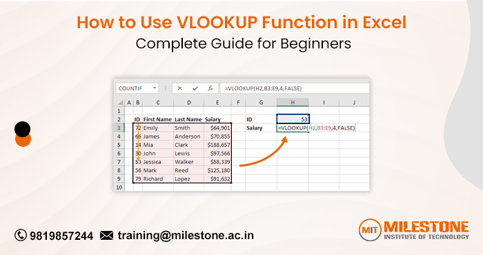
=VLOOKUP(lookup_value, table_array, col_index_num, [range_lookup])
Breakdown of Parameters:
- lookup_value The value that you wish to look for.
- table_array: The range of data where VLOOKUP will search.
- col_index_num: The table column from which the value should be obtained.
- range_lookup: A logical value (TRUE or FALSE). If TRUE, VLOOKUP returns the closest match. If FALSE, it returns an exact match.
How to Use VLOOKUP Function in Excel: Step-by-Step
To better understand VLOOKUP and how to use VLOOKUP Function in Excel, let’s go through an example. Suppose you have a table of employee data and want to find an employee’s department based on their ID.
Example:
You have the following data in cells A1 to C5:
| Employee ID | Name | Department |
| 101 | Raj Sawant | HR |
| 102 | Shruti Dhuri | IT |
| 103 | Gauri Deshpande | Marketing |
| 104 | Ishan Sharma | Finance |
You want to find the department of the employee with ID 103.
Step 1: Identify the Lookup Value
The lookup_value is the value you want to search for, which is 103 (Employee ID).
Step 2: Define the Table Array
The table_array refers to the range of cells that contains the data you want to search. In this case, it’s A1:C5, where Column A contains the Employee ID, Column B contains the Name, and Column C contains the Department.
Step 3: Specify the Column Index
The col_index_num represents the column number in the table array from which you want to return a value. Since we are looking for the Department, which is in Column C, the column index number is 3.
Step 4: Choose the Range Lookup
Since we want an exact match for Employee ID 103, we will set range_lookup to FALSE.
Step 5: Enter the Formula
Now, you can enter the formula in the desired cell:
=VLOOKUP(103, A1:C5, 3, FALSE)
The result will be Marketing, which is the department for Employee ID 103.
Best Practices for Using VLOOKUP
1. Ensure Your Data is Organized Vertically
VLOOKUP only works when your data is organized vertically, meaning the values you’re searching for must be in the first column of your table. If your data is horizontal, you will need to rearrange it or use a different function like HLOOKUP.
2. Use Absolute References for Table Array
When working with large datasets or copying the VLOOKUP formula to multiple cells, always use absolute references for the table array (e.g., $A$1:$C$5). This ensures that the table array remains constant as you drag the formula across different cells.
Example:
=VLOOKUP(103, $A$1:$C$5, 3, FALSE)
3. Check for Exact Matches
Range_lookup needs to be set to FALSE at all times if you’re searching for an exact match. If you leave it blank or set it to TRUE, Excel will look for the closest match, which can result in errors when dealing with non-sorted data.
4. Handle Errors with IFERROR
Sometimes, VLOOKUP may not find the value you are searching for, resulting in a #N/A error. To handle this gracefully, use the IFERROR function to display a custom message or an alternative value.
Example:
=IFERROR(VLOOKUP(103, $A$1:$C$5, 3, FALSE), “Not Found”)
If Employee ID 103 is not found, this formula will return “Not Found” instead of displaying an error.
5. Sort Your Data for Approximate Matches
If you’re using VLOOKUP with an approximate match (range_lookup = TRUE), ensure that the first column of your table array is sorted in ascending order. This helps VLOOKUP return the correct value when an exact match is not found.
6. Use Named Ranges for Readability
Instead of using cell references in your VLOOKUP formula, you can define a named range for your table array. This improves readability, especially when working with large datasets.
For example, define the range A1:C5 as EmployeeData, then your formula becomes:
=VLOOKUP(103, EmployeeData, 3, FALSE)
VLOOKUP vs. Other Lookup Functions
VLOOKUP is a powerful function, but it has limitations. It operates vertically and is limited to searching for values in a table’s first column. In some cases, other Excel functions like INDEX and MATCH or XLOOKUP (in Excel 2019 and Microsoft 365) may be more flexible.
INDEX and MATCH
Unlike VLOOKUP, the combination of INDEX and MATCH allows you to perform lookups both vertically and horizontally. Here’s an example of how you can use INDEX and MATCH to look up a department:
=INDEX(C1:C5, MATCH(103, A1:A5, 0))
In this case, MATCH(103, A1:A5, 0) finds the position of 103 in Column A, and INDEX(C1:C5, …) returns the corresponding value from Column C.
XLOOKUP
XLOOKUP is a more versatile alternative to VLOOKUP introduced in Microsoft Excel 2019 and Microsoft 365. It can search both vertically and horizontally, supports exact and approximate matches, and allows for returning results from any direction. Here’s an example of the same search for Employee ID 103 using XLOOKUP:
=XLOOKUP(103, A1:A5, C1:C5)
XLOOKUP eliminates the need for specifying a column index and handles errors more elegantly.
Common VLOOKUP Errors and Their Solutions
1. #N/A Error
The #N/A error occurs when VLOOKUP cannot find the lookup value in the first column. This may happen if the lookup value is misspelled, or there’s no exact match. To fix this, ensure that your lookup value is correct and matches the data format (e.g., text vs. numbers).
2. #REF! Error
The #REF! When col_index_num is more than the number of columns in the table array, an error is raised. To fix this, make sure that the column index is within the range of the table array.
3. #VALUE! Error
The #VALUE! error may occur if the lookup_value is a text string, but the table contains numbers, or vice versa. Make sure the table array and your lookup value have the same data types.
Advanced VLOOKUP Techniques
1. Multiple Criteria Lookup
VLOOKUP alone can’t handle multiple criteria, but you can combine it with other functions like CONCATENATE or the & operator. For example, if you want to look up based on both Employee ID and Name, you can create a new column that concatenates both values and use VLOOKUP on that column.
2. Two-Way Lookup
You can use VLOOKUP in combination with MATCH to perform two-way lookups. For example, if you have a table with products and regions and want to find the sales figure for a specific product and region, you can use MATCH to dynamically determine the column index.
Learn VLOOKUP Function for Data Analysis
Your ability to analyze data in Excel may be considerably improved by learning VLOOKUP. Mastering it will allow you to quickly and efficiently handle large datasets, perform lookups, and manipulate data with ease. If you’re looking to improve your Excel expertise and become a professional data analyst there are a lot of training centers and institutes which provide different courses. As per the research and reviews Milestone Institute of Technology is one of the popular institutes which provides data science and data analytics courses. Their comprehensive data analytics and data science programs cover all the essential topics, which every individual needs to master.
Frequently Asked Questions (FAQs)
Can VLOOKUP search for values located to the left of the lookup column?
No, VLOOKUP can only search for values in columns to the right of the lookup column. If you need to perform a leftward lookup, you can use a combination of INDEX and MATCH or consider using XLOOKUP.
What is the difference between VLOOKUP and HLOOKUP?
VLOOKUP searches vertically in columns, while HLOOKUP (Horizontal Lookup) searches horizontally in rows. HLOOKUP is used when your data is organized in a row-wise fashion.
Can VLOOKUP work with approximate matches?
Yes, VLOOKUP can work with approximate matches if the range_lookup parameter is set to TRUE. However, it’s important to ensure that the first column of your data is sorted in ascending order for accurate results. By mastering VLOOKUP and understanding its nuances, you can take your data analysis skills to the next level, making Excel an even more powerful tool in your workflow.